Spreadsheets
Exercise #1 | Exercise #2 | Exercise #3 | Exercise #4A | Exercise #4B | Exercise #5 | Exercise #5b | Excel Exercises Part 2
Microsoft Office includes a spreadsheet application called Excel. In this series of exercises you will explore the capabilities of this program.
1. Creating a Worksheet with Excel - page 197 Activity
Duplicate the spreadsheet shown on this page. Be sure to use formulas for the calculated values.
Create a pie chart and embed it into the spreadsheet.
Add a header with your name and date.
Show the spreadsheet to your instructor for teacher check.3. Payroll - see instructor for handout
4. Working with mutliple sheets - formatting cells, stretching, autosum, autofill, formulas - Watch the Lynda.com video - Excel 2013 Essential Training with Dennis Taylor - Chapter 14 - Data Analysis Tools
Creating a "What If" Table - Monthly Payments Table
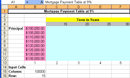
A "what if" table performs calculations using multiple inputs, in this exercise you will calculate the monthly mortgage payment based on differing loan amounts and length of the loan. Duplicate the following table:
In cell B4 insert the following formula: =PMT(0.09/12,B16*12,-B15)
The PMT formula calculates the payment for a loan based on the interest rate, principal amount (amount borrowed) and the length of the loan. In the above equation the interest rate is 9% (0.09) but since we want monthly payments the interest rate needs to be divided by 12 (/12). Next comes the number of payments, in this case the loan is for 15 years (cell B16) times 12 months. The last value is the amount of the loan (cell B15). Once you hit enter you should see a value of $1,014.27. On a 15 year loan of $100,000 at a 9% interest rate the monthly payment will be $1,014.27The next step is to have excel perform this same calculation for different principal amounts and different loan lengths. Select the entire table (B4 to F12) by clicking on B4 and dragging to F12. Click on the Data tab and then click on the What-If Analysis pull down list and select Data Table. An input window pops up asking for the row and column input values, enter B16 for the row input value and B15 for the column input value and click OK. What happens?
Create a copy of this sheet by clicking on the sheet tab at the bottom of the sheet and right click and select Move or Copy Sheet) and rename it 6 Percent. Modify your formula so this sheet shows the monthly payments for loans that are at 6 percent instead of 9%.
4B. Watch the Lynda.com video - Excel 2013: Essential Training with Dennis Taylor - Chapter 10 - If, VLOOKUP, and Power Functions - Get approximate table data with the VLOOKUP function.
VLookup Function - in this exercise you will create another table that automatically calculates the loan amount based on the table you already created in exercise 4A. Create the following table just below your current table (refer to the row and column numbers).
Enter a formula for the mortgage amount (the home price - down payment).
In the 25 years column use the following formula =VLOOKUP(E21,$B$5:$F$12,$E$13)
E21 is the mortgage amount, B5-F12 is the table and E13 is the column that should be searched (the column for a 25 year loan). The $ symbol in front of these cell locations makes them absolute references, they will not change when you copy this formula for the rest of the customers.Once you have completed this table copy it to your 6 % sheet to see what values would result at this lower rate.
Add a header with your name and date and print up both sheets.
5. Excel as a Database
In this exercise you will make use of the database capabilities of excel. Copy (use the copy and paste commands, do NOT type in these values) the following table into excel and save the list as AddressBook
Barnes Leanne 808 Summer Street Anaheim 63403 (213)555-4987 Brown Miles 154 Newburg Road Anaheim 63403 (213)555-4837 Griffith Stuart 1551 Dean Street Beverly Hills 62103 (213)555-3010 Moon Michael 17 Pine Street Beverly Hills 62103 (213)555-9275 Smith Trina 3954 Wood Avenue Anaheim 63402 (213)555-7283 Smith Sheila 417 Specific Court North Hollywood 65104 (213)555-9174 Walker Bette 1584 F Street North Hollywood 65102 (213)555-8129 Castillo Carl 1956 Park Avenue North Hollywood 65104 (213)555-5192 Davis John P.O. Box 2333 North Hollywood 65102 (213)555-8129 Dixon Amy 237 Albee Street North Hollywood 65102 (213)555-8917 Sort the table based on Last name. Go to the Data tab and click on the Sort button. Sort by last name then first name. Rename this sheet Last.
Copy the Last sheet and rename the new sheet City. Sort this sheet by City, Last name, first name.
Copy the Last sheet and rename it Zip. Sort this sheet by Zip and Last Name. Save your file.
Copy the Last sheet and rename it Filter City. Use the filter function (go to the Data tab and click on the Filter button) to only show people who live in Anaheim.
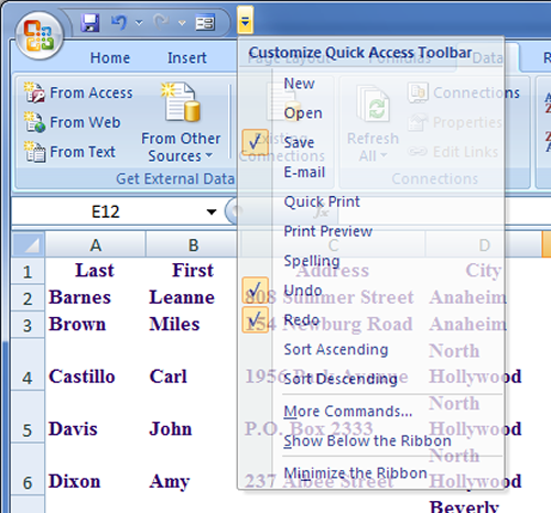
Turn the filter function off by clicking on the filter button again. Next you will use a form to enter data into your table. Forms are typically created for people who are not faimilar with Excel so they can quickly enter new data. To use the form function you will need to add a quick access button. Go to the top left corner of excell and you will see several quick access buttons (save, redo...)
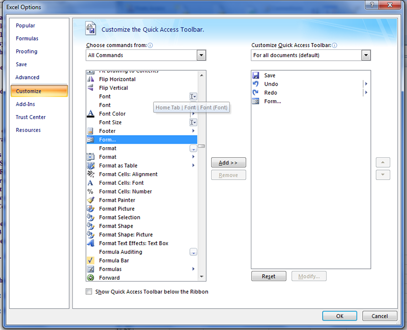
At the end of this row of buttons you will see a down arrow, click on this arrow to reveal a pull down menu. From this menu select "More Commands" and then choose All Commands in the "Choose Commands from:" and find the Form command.
Select the form command and then click on the Add button in the middle of your screen. Click on the OK button and then click on the new Form button that is now in your quick access tool bar. Use this form to enter a new row of data into the table.
5B Mail Merge using an Excel Database
Use the AddressBook table and the mail merge function of Word to create envelopes for each person in this list. Do NOT print out the labels, show them to your instructor for teacher check.
1. Open Word. Which tab should you select to access the mail merge function? Click on this tabl and then click on the Start Mail Merge button. From the pull down list choose Envelopes. Accept the default values in the Envelope Options window.
2. Your page view should now look like an envelope. Next click on the Select Recipients button and select Use Existing List. Browse to your AddressBook excel sheet (be sure the document is not currently open). Notice that several new buttons are now available in the Mailings tab.
3. Move your cursor to the middle of the envelope and then click on the Address Block button. Accept the defualt options provided and click OK. What appears in the middle of your envelope?
4. Click on the Finish & Merge button and select Edit Individual Documents and select the defaul on the next window. Show the envelopes to your instructor for teacher check.
Show the excel file and the labels to your instructor for teacher check.
Excel Exercises Part 2


